Data Analysis
1. Observables: Traditional vs Chemical Fingerprints
The choice of desciprtor can be crutial in determining the physical and chemical properties of small molecules. Two sets of descriptors, traditional and chemical fingerprints, were chosen and tested with lieaner regression in estimating partition coefficient. The former one consists of eight dependent vsariables, namely molecular weight, hydrogon bond donor, hydrogon bond acceptor, rotational bond number, total ring number, aromatic ring number, total charge and surface area. Thes e quantities can be obtained directly by the rdkit package with MOL or SMILES code as an input.
        # mol weight
        Wgt=Chem.rdMolDescriptors.CalcExactMolWt(mol)
        # HB acceptor and donor
        HBA=Chem.rdMolDescriptors.CalcNumHBA(mol)
        HBD=Chem.rdMolDescriptors.CalcNumHBD(mol)
        # Rotatable bonds
        RotBond=Lipinski.NumRotatableBonds(mol)
        # number of rings and aromatic rings
        Ring=Lipinski.RingCount(mol)
        AroRing=Lipinski.NumAromaticRings(mol)
        # Formal charge of the mol
        Charge=Chem.GetFormalCharge(mol)
        # Mol surface area
        Surf=Chem.MolSurf.pyLabuteASA(mol, includeHs=0)
On the other hand, Morgan/circular chemical fingerprints were also prepared at radius of 2 and 1024 bits.[1] The hashed fingerprints were generated in a manner demonstrated in Figure 4.

Figure 4: Illustrative Fingerprints with Ibuprofen
The linear regression fitting results using the two sets of observables were shown in Figure 5 and Figure 6. While both had R2 score between 0.6 and 0.7, linear regression with tranditional variables showed tendency to overestimate the partition coefficient, resulting in larger root-mean-squre deviation(RMSE). Such observables suffer from the following two flaws: 1. They are not mutually exclusive, for example, molecules of larger weight are also of larger suface area. 2. They can hardly be used to capture molecular similariry, due to its ambiguity. In cases where the chemical property of interest involves specific interaction, or on the other words, is more sensitive to the molecular similarity, using there observables may lead to further failure.
R2 score = 0.62; RMSE = 2.01
Mean score with five-fold cross-validation = 0.59 (+/- 0.09)

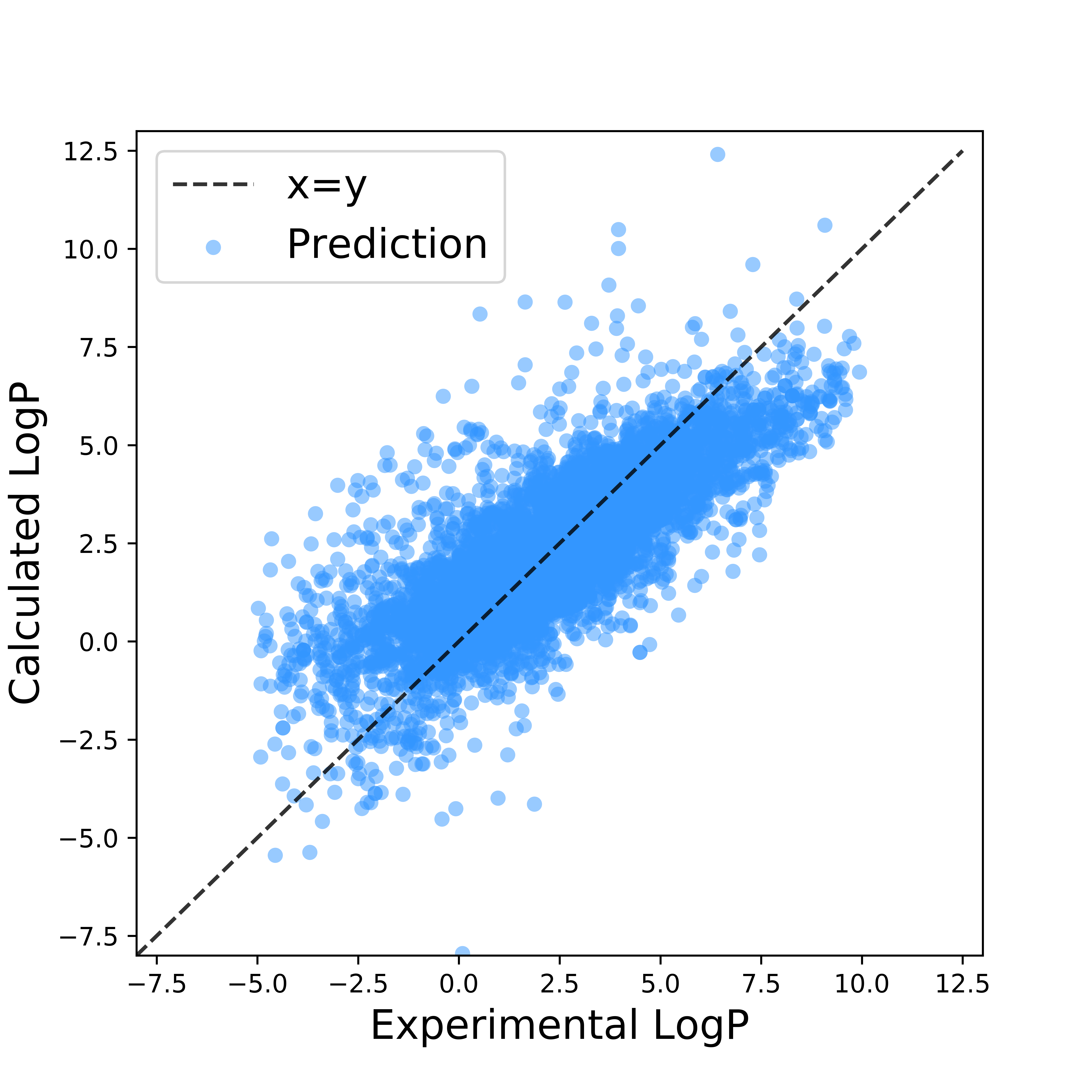
R2 score = 0.65; RMSE = 1.86
Mean score with five-fold cross-validation = 0.60 (+/- 0.08)
2. Partition Coefficient Fitting: Linear Regression vs Ridge vs Deep Neural Network
Figure 6 shows the linear regression results and Figure 7 shows the absolute coefficient value for each independent variables. Ranging in [-1,1], the coefficients all fall in the same magnitude indicating a good linear property of the dependent variable. Ridge model was also tested after a ten-step alpha scan in log space. The best model with shrinkage penalty at 0.1 was used for actual fitting, resulting in very similar performance as linear regression. (R2 score = 0.65; RMSE = 1.86; Mean score with five-fold cross-validation = 0.61 (+/- 0.08).) Deep neural network (DNN) has also been applied with three models: 1 layer with 500 neurons, 1 layer with 1000 neurons and 2 layers with 500 and 50 neurons. The fitting results along with the elaspsed time were shown in Figure 8-10. It is interesting to find that reducing the neurons from input has negative impact on the fitting results and increasing the number of layers improved the results marginally. This is in line with the previous discussion on the linearity nature of the problem.


R2 score = 0.71; RMSE = 1.56
Elaspsed time = 13.51 sec

R2 score = 0.76; RMSE = 1.28
Elaspsed time = 38.65 sec

R2 score = 0.75; RMSE = 1.30
Elaspsed time = 40.40 sec
3. Toxicity Estimation
It is very challenging even for chemistry experts to tell which of the two molecules in Figure 10 is toxic. While the left-hand side one is an effective ingredient in painkillers such as Tylenol and Panadol, the right-hand side molecule causes skin, eye and respiratory irritations. It also has specific target organ toxicity on single exposure. In drug development, huge amount of efforts are dedicated to the toxicity test in pre-clinical and clinical trails. Accurate prediction on the toxicity property of potential drug molecules can greatly reduce the failure rate, thus bring down the total cost for each drug that eventually made to the market.
Based on previous discussions, chemical fingerprints can serve as observables in toxicity prediction. Figure 11 shows the two datasets used in this study, 3380 FDA approved benign drug molecules and 3180 toxic drug-like molecules after data cleaning. [2] The two classes were combined and fitted with logistic regression. The results are listed in Table 1. Testing on 760 molecules ended up with an overall accuracy of 95.4%.
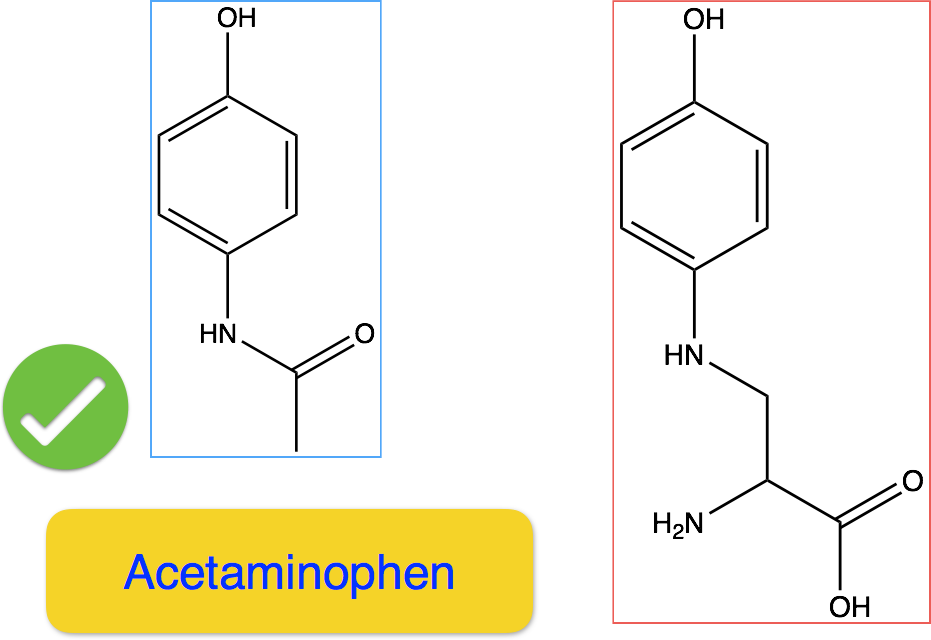
Figure 10: Acetominophen and the Counterparts

| Predicted benign | Predicted toxic | |
|---|---|---|
| Experimentally toxic | 8.4% | 91.6% |
| Experimentally benign | 99.2% | 0.8% |
4. Potential Cost Saving in Drug Development
On average, the toxicity test for each successful drug would cost around $400 M, about 25% of the total cost. Roughly 60% of the drug candidate would be excluded due to toxicity or side effect in the pre-clinical step. With the aforementioned algorithm, about 95% toxic candidates can be scrutinized before the animal test, thus potentially save around $230 M for each successful drug.
Reference:
[1]. Rogers, D.; Hahn, M. Extended-Connectivity Fingerprints. J. Chem. Inf. Model. 2010, 50 (5), 742–754.
[2]. http://bioinformatics.charite.de/supertoxic/index.php?site=browse_toxins